
PID control (Proportional-Integral-Derivative) is a major building block of a robotic system. It provides a straight-forward method to precisely control a motor to perform a pre-determined action without the need for direct human control to adjust the machine. PID control is an algorithm that uses a determined error that can be used calculate the necessary motor response to achieve your task.
Open Loop Versus Closed Loop
Open loop control is simple. With open loop control your input is in direct control of the output, meaning that whatever the input states occurs at the output. The drawback to this is that there is no feedback mechanism. Sure, your widget is doing exactly what you told it to but there’s no true way to know that what it’s doing is accurate. This is where closed loop comes in. With a closed loop system you receive feedback from your system so that you can adjust your input so that your system performs exactly what you intended. This is the basis of PID control.
Basic Theory
The image below is a block diagram of a PID controller in a feedback loop. The loop begins in the top right where we compare our current position y(t) and our desired position r(t) to determine the error in our system. This error is then sent to our PID control. This is broken down into three parts. The first is the proportional component where we multiply our error by a constant. This is the primary component of the PID where we correct our present error. It gives us our base correction factor that is then refined in the next two parts. Next is the integral component. With this we integrate our error over time which corrects our steady-state error. Lastly, we have our derivative component where we take action on sudden changes. This is greatly useful when having a robot perform something like line following. It will correct for sudden changes of the track. These three components are then summed and fed into our process so that the robot can perform the necessary adjustment.
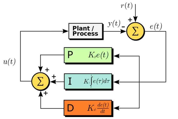
PID Diagram. Image Courtesy of Wikipedia
Tuning
To achieve smooth and precise behaviour, it will be necessary to manually tune the PID until we get the results that we’re looking for. The chart below will show the effects of increasing each parameter independently. The general manual tuning process would be the tune your proportional constant until you start to notice oscillation. Once oscillation is seen, reduce it by half and increase your integral constant until your behaviour is satisfactory. Once you’ve tuned the PID under a steady state condition the derivative constant should then be increased until you receive the response time you’re looking for.
In practical applications, you may be able to largely tune your PID using entirely the P constant. If there is a need for quick corrections you will need to increase the derivative constant until you get the performance you’re looking for. Fine tuning the integral constant may, or may not, be necessary.
| Parameter | Rise Time | Overshoot | Settling Time | Steady-state error | Stability |
|---|---|---|---|---|---|
| Kp | Decrease | Increase | Small Change | Decrease | Degrade |
| Ki | Decrease | Increase | Increase | Eliminate | Degrade |
| Kd | Minor change | Decrease | Decrease | No effect in theory | Can Improve |
Application Example: The Servo
A basic application of PID control is the servo. A servo is a motor with a feedback sensor such as a resistive potentiometer. When commanded to a position it compares the command position to the current value of the potentiometer and adjusts motor power until they are equivalent. In the example code below I will use a Syren 10A (TE-098-110) motor controller to position one of our IG32 motors based on the value of one of our two axis joysticks (TE-128-002).
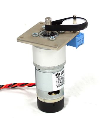
Servo Test Jig
// ****************************************************
// Libraries
// ****************************************************
#include
#include
// ****************************************************
// Hardware Pin Definitions
// ****************************************************
#define S_ESTOP 10
#define S_RX 9
#define SENSOR A0
#define COMMAND A1
// ****************************************************
// Hardware Pin Definitions
// ****************************************************
const float Kp = 0.5;
const float Ki = 0.03;
const float Kd = 0.0;
int errorArray[60];
int k = 0;
int lastError;
// ****************************************************
// Motor Controller Declarations
// ****************************************************
SoftwareSerial SWSerial(NOT_A_PIN, S_RX); // RX on no pin (unused), TX on pin 11 (to S1).
Sabertooth ST(128, SWSerial); // Address 128, and use SWSerial as the serial port.
// ****************************************************
// Initial setup function, called once
// RETURNS: none
// ****************************************************
void setup() {
int i;
// Initialize serial
Serial.begin(9600); // Debug serial output
SWSerial.begin(9600); // Syren Interface
// Initialize connected I/O
pinMode(S_ESTOP, OUTPUT);
digitalWrite(S_ESTOP, HIGH); // Release motor controller ESTOP
// Initialize Motor Controller
ST.autobaud(); // Sends Hex 0xAA to determine expected baud rate
for (i=0; i<=60; i++) { errorArray = 0; } } // **************************************************** // Main program loop // RETURNS: none // **************************************************** void loop() { int sensorValue; int commandValue; int positionError; int motorValue; int i; long runningSum = 0; int PID; float PIDp; float PIDi; float PIDd; sensorValue = analogRead(SENSOR); // Our actual position commandValue = analogRead(COMMAND); // Position we need to go to // Determine our error positionError = sensorValue - commandValue; // Apply our P constant PIDp = positionError * Kp; errorArray[k] = positionError; k = k+1; if (k >= 60)
k = 0;
// Calculate the integral contribution
for (i = 0; i < 60; i++) {
runningSum = runningSum + errorArray;
}
PIDi = runningSum * Ki;
// Calculate the derivative contribution
PIDd = positionError - lastError;
PIDd = Kd * PIDd;
PIDd = PIDd / 100; // Approximately 100ms since last compute
lastError = positionError;
// Apply the integral and derivative components
PID = PIDp + PIDi + PIDd;
// Assign our PID output to our motor value
motorValue = PID;
// Bound our motor values. Our motor controller is expecting a value
// of -127 to 127
if (motorValue < -127) motorValue = -127; if (motorValue > 127)
motorValue = 127;
// Command our Motor Controller
ST.motor(motorValue);
// Debug Output
Serial.print("Concerns and Variations
Not all applications can be solved with a simple PID. For example, when designing a control system for a robotic arm loading and gravity will have a significant effect on motor power and movement. When an arm his holding something it will take significantly more power to move the arm up versus down. In cases like this you will need to employ a more robust PID scheme and more complicated algorithms.
#techthursday #PID